When I was in high school, two cool things that I learned from physics were “vectors” and “calculus”. I was (and am still) awestruck by following statement
Uniform circular motion is an accelerated motion.
At college, during my first (and second last) physics course, I was taught “vector calculus” and I didn’t enjoy it. Last year I learned “linear algebra”, that is the study of vector spaces, matrices, linear transformations… Also, a few months ago I wrote about my understanding of Algebra. In it I briefly mentioned that “…study of symmetry of equations, geometric objects, etc. became one of the central topics of interest…” and this lead to what we call “Abstract Algebra” of which linear algebra is a part. Following video by 3blue1brown explains how our understanding of vectors from physics can be used to develop the subject of linear algebra.
But, one should ask : “Why do we care to classify physical quantities as scalars and vectors?”. The answer to this question lies in the quest of physics to find the invariants, in terms of which we can state the Laws of nature. In general, the idea of finding invariants is a useful problem solving strategy in mathematics (the language of physics). For example, consider following problem from the book “Problem-Solving Strategies” by Arthur Engel:
Suppose the positive integer n is odd. The numbers 1,2,…, 2n are written on the blackboard. Then one can pick any two numbers a and b, erase them and write instead |a-b|. Prove that an odd number will remain at the end.
To prove this statement, one will have to use the concept of “parity” of the sum 1+2+3+…+2n as the invariant. And as stated in the video above, vectors are invariant under transformations of coordinate systems (the components change, but length and direction of arrow remain unchanged). For example, consider the rotation of 2D axis by angle θ, keeping the origin fixed.

By Guy vandegrift (Own work) [CC BY-SA 3.0], via Wikimedia Commons

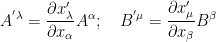
Now, we can rewrite this by using 


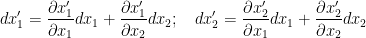
Now we differentiate this system of equations to get:
where 

for 


for 


But, there are physical quantities which can’t be classified as scalar or vector. For example, “stress”: the internal force experienced by a material due to the “strain” caused by external force; is described as a “tensor of rank 2”. This is so, because the stress at any point on the surface depends upon the external force vector and area vector i.e. it describes things happening due to interaction between two vectors. The Cauchy stress tensor 


where 


![\boldsymbol{\sigma} = \left[{\begin{matrix} \mathbf{T}^{(\mathbf{e}_1)} \\ \mathbf{T}^{(\mathbf{e}_2)} \\ \mathbf{T}^{(\mathbf{e}_3)} \\ \end{matrix}}\right] = \left[{\begin{matrix} \sigma _{11} & \sigma _{12} & \sigma _{13} \\ \sigma _{21} & \sigma _{22} & \sigma _{23} \\ \sigma _{31} & \sigma _{32} & \sigma _{33} \\ \end{matrix}}\right]](https://s0.wp.com/latex.php?latex=%5Cboldsymbol%7B%5Csigma%7D+%3D+%5Cleft%5B%7B%5Cbegin%7Bmatrix%7D+%5Cmathbf%7BT%7D%5E%7B%28%5Cmathbf%7Be%7D_1%29%7D+%5C%5C%C2%A0+%5Cmathbf%7BT%7D%5E%7B%28%5Cmathbf%7Be%7D_2%29%7D+%5C%5C%C2%A0+%5Cmathbf%7BT%7D%5E%7B%28%5Cmathbf%7Be%7D_3%29%7D+%5C%5C%C2%A0+%5Cend%7Bmatrix%7D%7D%5Cright%5D+%3D%C2%A0+%5Cleft%5B%7B%5Cbegin%7Bmatrix%7D%C2%A0+%5Csigma+_%7B11%7D+%26+%5Csigma+_%7B12%7D+%26+%5Csigma+_%7B13%7D+%5C%5C%C2%A0+%5Csigma+_%7B21%7D+%26+%5Csigma+_%7B22%7D+%26+%5Csigma+_%7B23%7D+%5C%5C%C2%A0+%5Csigma+_%7B31%7D+%26+%5Csigma+_%7B32%7D+%26+%5Csigma+_%7B33%7D+%5C%5C%C2%A0+%5Cend%7Bmatrix%7D%7D%5Cright%5D&bg=ffffff&fg=000000&s=0&c=20201002)

By Sanpaz (Own work) [CC BY-SA 3.0 or GFDL], via Wikimedia Commons
In this terminology, a scalar is a tensor of rank zero and a vector is a tensor of rank one. Moreover, in an n-dimensional space:
- a vector has n components
- a tensor of rank two has n^2 components
- a tensor of rank three has n^3 components
- and so on …
Just like vectors, tensors in general are invariant under transformations of coordinate systems. We wish to exploit this further. Let’s reconsider the boxed equation stated earlier. Since we are working with Euclidean metric i.e the length s of vector is given by 


where 
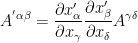
where the sum is over the indices 


So, we just analysed the invariance of one of the flavours of tensors. Mathematically thinking, one should expect existence of something “like algebraic inverse” of contravariant tensor because tensor is a generalization of vector and in linear algebra we study inverse operations. Let’s consider a situation when we want to analyse density of an object at different points. For simplicity, lets’ consider a point 

A surface whose density is different in different parts
If we designate by 


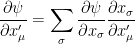
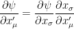
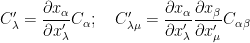
Now our motive is to express 


Here we have used the idea that if x,y, z are three variables such that y and z depend on x and the calculation of the change in z per unit change in x NOT easy, then we can calculate it using: 
for
for 


where 

where the sum is over the indices
Comparing the (boxed) equations describing contravariant and covariant vectors, we observe that the coefficients on the right are reciprocal of each other (as promised…). Moreover, all these boxed equations represent the law of transformation for tensors of rank one (a.k.a. vectors), which can be generalized to a tensor of any rank.
Our final task is to see how these two flavours of tensors interact with each other. Let’s study the algebraic operations of addition and multiplication for both flavours of tensors, just like the way we did for vectors (note that vector product = dot product, because cross product can’t be generalized to n-dimensional vectors).
First consider the case of contravariant tensors. Let 


for 

for
For the case of covariant tensors, the addition and (outer) multiplication is done in same manner as above. Let 


for
for
Now, as promised, it’s the time to see how both of these flavours of tensors interact with each other. Let’s extend the notion of outer multiplication defined for each flavour of tensor, to outer product of a contravariant tensor with a covariant tensor. For example, consider vectors (a.k.a. tensors of rank 1) of each type:

then their outer product leads to

where 
In general, if two mixed tensors of rank m (having 


Unlike the previous two types of tensors, we can’t illustrate it using a simple physical example. To convince yourself, consider following two mixed tensors of rank 3 and rank 2, respectively:

then following the notations introduced, their outer product is of rank 5 and is given by
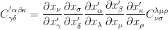
Behind this notation, the processes are really complicated. Now, suppose that we are working in 3D vector space. Then, the transformation law for tensor 


So, unlike previous two cases of contravarient and covariant tensors, the proof of outer product of mixed tens;ors is rather complicated and out of scope for discussion in this introductory post.
Reference:
[L] Lillian R. Lieber, The Einstein Theory of Relativity. Internet Archive: https://archive.org/details/einsteintheoryof032414mbp
 . I personally don’t like this name because all of mathematics is man/woman made, hence all mathematical objects are imaginary (there is no perfect circle in nature…) and lack physical meaning. Moreover, these numbers are very useful in physics (a.k.a. the study of nature using mathematics). For example, “time-dependent
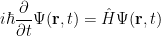


 of
of  , in a manner exactly analogous to the definition of the standard unit circle in
  . Apparently U is some sort of surface in
  and
and  then by setting
  we get the circle
  in x-u plane for v=0 and the hyperbola
  in x-vi plane for u=0.
 and
and  in
in 
 consisting of the non-negative imaginary axis and the numbers with a positive real part. Therefore, the complex distance between two points in
 with
with  , while if it is below the x axis, its radian measure is
  . As in the real case, we define
  and
and  to be the z and w coordinates of p. According to above figure (b), this gives

 , and are in agreement with the expansions of
  and
and  stated earlier.
 .
. through u is span(u), which is
  passing through a nonzero vector u can be defined as the set of all nonnegative real multiples of u. Extending this to
  .
. and
and  .
. counts the number of representations of
  by
by  squares, allowing zeros and distinguishing signs and order.
 can be written as sum of two squares if and only if it is can be written as
  for some integer
  such that
  is divisible by 2017.
 is divisible by 2017. Since half of the residues modulo 2017 are quadratic non-residue, it’s easy to check our guess using
  is smallest solution (in fact here is the
  , we get
  .
. using the
  where
where  .
. is
is  . Hence, the norm of 229+i, N(229+i) = 52442. For euclidean algorithm I will use long division/calculator as:
 .
.
You must be logged in to post a comment.