Prove that if , then we do not have any nontrivial solutions of the equation where are rational functions. Solutions of the form where is a rational function and are complex numbers satisfying , are called trivial.
This problem is analogous to the Fermat’s Last Theorem (FLT) which states that for , has no nontrivial integer solutions.
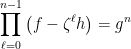
Since any rational solution yields a complex polynomial solution, by clearing the denominators, it is sufficient to assume that is a polynomial solution such that is minimal among all polynomial solutions, where .
Assume also that are relatively prime. Hence we have , i.e. . Now using the simple factorization identity involving the roots of unity, we get:
Now consider the factors . Note that, since , these elements belong to the 2-dimensional vector space generated by over . Hence these three elements are linearly dependent, i.e. there exists a vanishing linear combination with complex coefficients (not all zero) in these three elements. Thus there exist so that . We then set , and observe that .
Moreover, the polynomials for and since . Thus contradicting the minimality of , i.e. the minimal (degree) solution didn’t exist. Hence no solution exists.
The above argument fails for proving the non-existence of integer solutions since two coprime integers don’t form a 2-dimensional vector space over .
If you have spent some time with undergraduate mathematics, you would have probably heard the word “norm”. This term is encountered in various branches of mathematics, like (as per Wikipedia):
But, it seems to occur only in abstract algebra. Although the definition of this term is always algebraic, it has a topological interpretation when we are working with vector spaces. It secretly connects a vector space to a topological space where we can study differentiation (metric space), by satisfying the conditions of a metric. This point of view along with an inner product structure, is explored when we study functional analysis.
I want to talk about the algebraic and analytic differences between real and complex numbers. Firstly, let’s have a look at following beautiful explanation by Richard Feynman (from his QED lectures) about similarities between real and complex numbers:
Before reading this explanation, I used to believe that the need to establish “Fundamental theorem Algebra” (read this beautiful paper by Daniel J. Velleman to learn about proof of this theorem) was only way to motivate study of complex numbers.
The fundamental difference between real and complex numbers is
Real numbers form an ordered field, but complex numbers can’t form an ordered field. [Proof]
Where we define ordered field as follows:
Let be a field. Suppose that there is a set which satisfies the following properties:
For each , exactly one of the following statements holds: , , .
For , and .
If such a exists, then is an ordered field. Moreover, we define .
Note that, without retaining the vector space structure of complex numbers we CAN establish the order for complex numbers [Proof], but that is useless. I find this consequence pretty interesting, because though and are isomorphic as additive groups (and as vector spaces over ) but not isomorphic as rings (and hence not isomorphic as fields).
Now let’s have a look at the consequence of the difference between the two number systems due to the order structure.
Though both real and complex numbers form a complete field (a property of topological spaces), but only real numbers have least upper bound property.
Where we define least upper bound property as follows:
Let be a non-empty set of real numbers.
A real number is called an upper bound for if for all .
A real number is the least upper bound (or supremum) for if is an upper bound for and for every upper bound of .
The least-upper-bound property states that any non-empty set of real numbers that has an upper bound must have a least upper bound in real numbers.
This least upper bound property is referred to as Dedekind completeness. Therefore, though both and are complete as a metric space [proof] but only is Dedekind complete.
In an arbitrary ordered field one has the notion of Dedekind completeness — every nonempty bounded above subset has a least upper bound — and also the notion of sequential completeness — every Cauchy sequence converges. The main theorem relating these two notions of completeness is as follows [source]:
For an ordered field , the following are equivalent:
(i) is Dedekind complete.
(ii) is sequentially complete and Archimedean.
Where we defined an Archimedean field as an ordered field such that for each element there exists a finite expression whose value is greater than that element, that is, there are no infinite elements.
As remarked earlier, is not an ordered field and hence can’t be Archimedean. Therefore, can’t have least-upper-bound property, though it’s complete in topological sense. So, the consequence of all this is:
We can’t use complex numbers for counting.
But still, complex numbers are very important part of modern arithmetic (number-theory), because they enable us to view properties of numbers from a geometric point of view [source].
In several of my previous posts I have mentioned the word “dimension”. Recently I realized that dimension can be of two types, as pointed out by Bernhard Riemann in his famous lecture in 1854. Let me quote Donal O’Shea from pp. 99 of his book “The Poincaré Conjecture” :
Continuous spaces can have any dimension, and can even be infinite dimensional. One needs to distinguish between the notion of a space and a space with a geometry. The same space can have different geometries. A geometry is an additional structure on a space. Nowadays, we say that one must distinguish between topology and geometry.
[Here by the term “space(s)” the author means “topological space”]
In mathematics, the word “dimension” can have different meanings. But, broadly speaking, there are only three different ways of defining/thinking about “dimension”:
Dimension of Vector Space: It’s the number of elements in basis of the vector space. This is the sense in which the term dimension is used in geometry (while doing calculus) and algebra. For example:
A circle is a two dimensional object since we need a two dimensional vector space (aka coordinates) to write it. In general, this is how we define dimension for Euclidean space (which is an affine space, i.e. what is left of a vector space after you’ve forgotten which point is the origin).
Dimension of a differentiable manifold is the dimension of its tangent vector space at any point.
Dimension of a variety (an algebraic object) is the dimension of tangent vector space at any regular point. Krull dimension is remotely motivated by the idea of dimension of vector spaces.
Dimension of Topological Space: It’s the smallest integer that is somehow related to open sets in the given topological space. In contrast to a basis of a vector space, a basis of topological space need not be maximal; indeed, the only maximal base is the topology itself. Moreover, dimension is this case can be defined using “Lebesgue covering dimension” or in some nice cases using “Inductive dimension“. This is the sense in which the term dimension is used in topology. For example:
A circle is one dimensional object and a disc is two dimensional by topological definition of dimension.
Two spaces are said to have same dimension if and only if there exists a continuous bijective map between them. Due to this, a curve and a plane have different dimension even though curves can fill space. Space-filling curves are special cases of fractal constructions. No differentiable space-filling curve can exist. Roughly speaking, differentiability puts a bound on how fast the curve can turn.
Fractal Dimension: It’s a notion designed to study the complex sets/structures like fractals that allows notions of objects with dimensions other than integers. It’s definition lies in between of that of dimension of vector spaces and topological spaces. It can be defined in various similar ways. Most common way is to define it as “dimension of Hausdorff measure on a metric space” (measure theory enable us to integrate a function without worrying about its smoothness and the defining property of fractals is that they are NOT smooth). This sense of dimension is used in very specific cases. For example:
A curve with fractal dimension very near to 1, say 1.10, behaves quite like an ordinary line, but a curve with fractal dimension 1.9 winds convolutedly through space very nearly like a surface.
The fractal dimension of the Koch curve is , but its topological dimension is 1 (just like the space-filling curves). The Koch curve is continuous everywhere but differentiable nowhere.
The fractal dimension of space-filling curves is 2, but their topological dimension is 1. [source]
A surface with fractal dimension of 2.1 fills space very much like an ordinary surface, but one with a fractal dimension of 2.9 folds and flows to fill space rather nearly like a volume.
This simple observation has very interesting consequences. For example, consider the following statement from. pp. 167 of the book “The Poincaré Conjecture” by Donal O’Shea:
… there are infinitely many incompatible ways of doing calculus in four-space. This contrasts with every other dimension…
This leads to a natural question:
Why is it difficult to develop calculus for any in general?
Actually, if we consider as a vector space then developing calculus is not a big deal (as done in multivariable calculus). But, if we consider as a topological space then it becomes a challenging task due to the lack of required algebraic structure on the space. So, Donal O’Shea is actually pointing to the fact that doing calculus on differentiable manifolds in is difficult. And this is because we are considering as 4-dimensional topological space.
Now, I will end this post by pointing to the way in which definition of dimension should be seen in my older posts:
Dimension ≡ Dimension of the underlying vector space
When I was in high school, two cool things that I learned from physics were “vectors” and “calculus”. I was (and am still) awestruck by following statement
Uniform circular motion is an accelerated motion.
At college, during my first (and second last) physics course, I was taught “vector calculus” and I didn’t enjoy it. Last year I learned “linear algebra”, that is the study of vector spaces, matrices, linear transformations… Also, a few months ago I wrote about my understanding of Algebra. In it I briefly mentioned that “…study of symmetry of equations, geometric objects, etc. became one of the central topics of interest…” and this lead to what we call “Abstract Algebra” of which linear algebra is a part. Following video by 3blue1brown explains how our understanding of vectors from physics can be used to develop the subject of linear algebra.
But, one should ask : “Why do we care to classify physical quantities as scalars and vectors?”. The answer to this question lies in the quest of physics to find the invariants, in terms of which we can state the Laws of nature. In general, the idea of finding invariants is a useful problem solving strategy in mathematics (the language of physics). For example, consider following problem from the book “Problem-Solving Strategies” by Arthur Engel:
Suppose the positive integer n is odd. The numbers 1,2,…, 2n are written on the blackboard. Then one can pick any two numbers a and b, erase them and write instead |a-b|. Prove that an odd number will remain at the end.
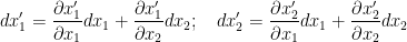
To prove this statement, one will have to use the concept of “parity” of the sum 1+2+3+…+2n as the invariant. And as stated in the video above, vectors are invariant under transformations of coordinate systems (the components change, but length and direction of arrow remain unchanged). For example, consider the rotation of 2D axis by angle θ, keeping the origin fixed.
Now, we can rewrite this by using and instead of and ; and putting different subscripts on the single letter instead of functions of :
Now we differentiate this system of equations to get:
where . We can rewrite this system in condensed form as:
for and . We can further abbreviate it by omitting the summation symbol with the understanding that whenever a subscript occurs twice in a single term, we do summation on that subscript.
for and . This equation represents ANY transformation of coordinates whenever the values of and are in one-to-one correspondence. Moreover, it can be extended to represent transformation of coordinates of any n-dimensional vector. For example, if and then it represents coordinate transformations of a 3-dimensional vector.
But, there are physical quantities which can’t be classified as scalar or vector. For example, “stress”: the internal force experienced by a material due to the “strain” caused by external force; is described as a “tensor of rank 2”. This is so, because the stress at any point on the surface depends upon the external force vector and area vector i.e. it describes things happening due to interaction between two vectors. The Cauchy stress tensor consists of nine components that completely define the state of stress at a point inside a material in the deformed state (where i corresponds to the force component direction and j corresponds to the area component direction). The tensor relates a unit-length direction vector n to the stress vector across an imaginary surface perpendicular to n:
where,
where , and are normal stresses, and , , , , and are shear stresses. We can represent the stress vector acting on a plane with normal unit vector n, as:
Here, the tetrahedron is formed by slicing a parallelepiped along an arbitrary plane n. So, the force acting on the plane n is the reaction exerted by the other half of the parallelepiped and has an opposite sign.
In this terminology, a scalar is a tensor of rank zero and a vector is a tensor of rank one. Moreover, in an n-dimensional space:
a vector has n components
a tensor of rank two has n^2 components
a tensor of rank three has n^3 components
and so on …
Just like vectors, tensors in general are invariant under transformations of coordinate systems. We wish to exploit this further. Let’s reconsider the boxed equation stated earlier. Since we are working with Euclidean metric i.e the length s of vector is given by , we have i.e. and are the components of . So, replacing and by and we get (motivation is to capture the idea of area vector)
where are components of a vector in certain coordinate system (note that superscripts are just for indexing purposes and do NOT represent exponents). Any set of quantities which transforms according to this equation is defined to be a contravariant vector . Moreover, we can generalize this equation to a tensor of any rank. For example, a contravariant tensor of rank two is defined by:
where the sum is over the indices and (since they occur twice in the term on right). We can illustrate this for 3 dimensional space, i.e. but summation performed only on and ; for instance, if and then we have:
So, we just analysed the invariance of one of the flavours of tensors. Mathematically thinking, one should expect existence of something “like algebraic inverse” of contravariant tensor because tensor is a generalization of vector and in linear algebra we study inverse operations. Let’s consider a situation when we want to analyse density of an object at different points. For simplicity, lets’ consider a point on a plane surface with variable density.
A surface whose density is different in different parts
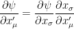
If we designate by the density at A, then and represent, respectively the partial variation of in the and directions. Although is a scalar quantity, the “change in ” is a directed quantity with components and . Note that, “change in ” is a tensor of rank one because it depends upon the various directions. But it’s a tensor in a sense different from what we saw in case of “stress”. This “difference” will become clear once we analyse what happens to this quantity when the coordinate system is changed.
Now our motive is to express , in terms of , . Note that, a change in will affect “both” and (as seen in rotation of 2D axis in case of vector). Hence, the resulting changes in and will affect
Here we have used the idea that if x,y, z are three variables such that y and z depend on x and the calculation of the change in z per unit change in x NOT easy, then we can calculate it using: . We can rewrite this system in condensed form as:
for and . We can further abbreviate it by omitting the summation symbol with the understanding that whenever a subscript occurs twice in a single term, we do summation on that subscript.
for and . Finally replacing by and by (to make it similar to notation introduced in case of stress tensor)
where are components of a vector in certain coordinate system. Any set of quantities which transforms according to this equation is defined to be a covariant vector . Moreover, we can generalize this equation to a tensor of any rank. For example, a covariant tensor of rank two is defined by:
where the sum is over the indices and (since they occur twice in the term on right).
Comparing the (boxed) equations describing contravariant and covariant vectors, we observe that the coefficients on the right are reciprocal of each other (as promised…). Moreover, all these boxed equations represent the law of transformation for tensors of rank one (a.k.a. vectors), which can be generalized to a tensor of any rank.
Our final task is to see how these two flavours of tensors interact with each other. Let’s study the algebraic operations of addition and multiplication for both flavours of tensors, just like the way we did for vectors (note that vector product = dot product, because cross product can’t be generalized to n-dimensional vectors).
First consider the case of contravariant tensors. Let be a vector having two components and in a plane and be another such vector. If we define and (this allows 4 components, namely ) with
for , then on their addition and multiplication (called outer multiplication) we get:
for . One can prove this by patiently multiplying each term and then rearranging them. In general, if two contravariant tensors of rank m and n respectively, are multiplied together, the result is a contravariant tensor of rank m+n.
For the case of covariant tensors, the addition and (outer) multiplication is done in same manner as above. Let be a vector having two components and in a plane and be another such vector. If we define and (this allows 4 components, namely ) with
for , then on their addition and multiplication (called outer multiplication) we get:
for . In general, if two covariant tensors of rank m and n respectively, are multiplied together, the result is a covariant tensor of rank m+n.
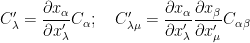
Now, as promised, it’s the time to see how both of these flavours of tensors interact with each other. Let’s extend the notion of outer multiplication defined for each flavour of tensor, to outer product of a contravariant tensor with a covariant tensor. For example, consider vectors (a.k.a. tensors of rank 1) of each type:
then their outer product leads to
where . This is neither a contravarient nor a covariant tensor, hence is rather called a mixed tensor of rank 2. More generally, if a contravariant tensor of rank m and a covariant tensor of rank n are multiplied together so as to form their outer product, the result is a mixed tensor of rank m+n.
In general, if two mixed tensors of rank m (having indices/superscripts of contravariance and indices/subscripts of covariance, such that ) and n (having indices/superscripts of contravariance and indices/subscripts of covariance, such that ) respectively, are multiplied together, the result is a mixed tensor of rank m+n (having indices/superscripts of contravariance and indices/subscripts of covariance, such that ) .
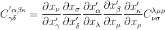
Unlike the previous two types of tensors, we can’t illustrate it using a simple physical example. To convince yourself, consider following two mixed tensors of rank 3 and rank 2, respectively:
then following the notations introduced, their outer product is of rank 5 and is given by
Behind this notation, the processes are really complicated. Now, suppose that we are working in 3D vector space. Then, the transformation law for tensor represents a set of 27 (=3^3) equations with each equation having 27 terms on the right. And the transformation law for tensor represents a set of 9 (=3^2) equations with each equation having 9 terms on the right. Therefore, the transformation law of their outer product tensor represents a set of 243 (=3^5) equations with each equation having 243 terms on the right.
So, unlike previous two cases of contravarient and covariant tensors, the proof of outer product of mixed tens;ors is rather complicated and out of scope for discussion in this introductory post.
, then we do not have any nontrivial solutions of the equation
where
are rational functions. Solutions of the form
where
is a rational function and
are complex numbers satisfying
, are called trivial.


![h_\ell = \sqrt[n]{a_\ell}g_\ell](https://s0.wp.com/latex.php?latex=h_%5Cell+%3D+%5Csqrt%5Bn%5D%7Ba_%5Cell%7Dg_%5Cell&bg=ffffff&fg=000000&s=0&c=20201002)


 be a field. Suppose that there is a set
  which satisfies the following properties:
 , exactly one of the following statements holds:
  ,
,  ,
,  .
. ,
,  and
and  .
. exists, then
  .
. and
and  ) but
) but  be a non-empty set of real numbers.
 is called an upper bound for
  for all
  .
. for every upper bound
  of
of  whose value is greater than that element, that is, there are no infinite elements.
 , but its topological dimension is 1 (just like the space-filling curves). The Koch curve is continuous everywhere but differentiable nowhere.
 in general?
 is difficult. And this is because we are considering

 and
and  instead of
  instead of functions of
  :
:
 . We can rewrite this system in condensed form as:
 and
and  . We can further abbreviate it by omitting the summation symbol
  with the understanding that whenever a subscript occurs twice in a single term, we do summation on that subscript.
 and
and  are in one-to-one correspondence. Moreover, it can be extended to represent transformation of coordinates of any n-dimensional vector. For example, if
  and
and  then it represents coordinate transformations of a 3-dimensional vector.
 consists of nine components
  that completely define the state of stress at a point inside a material in the deformed state (where i corresponds to the force component direction and j corresponds to the area component direction). The tensor relates a unit-length direction vector n to the stress vector
  across an imaginary surface perpendicular to n:
 where,
 ![\boldsymbol{\sigma} = \left[{\begin{matrix} \mathbf{T}^{(\mathbf{e}_1)} \\ \mathbf{T}^{(\mathbf{e}_2)} \\ \mathbf{T}^{(\mathbf{e}_3)} \\ \end{matrix}}\right] = \left[{\begin{matrix} \sigma _{11} & \sigma _{12} & \sigma _{13} \\ \sigma _{21} & \sigma _{22} & \sigma _{23} \\ \sigma _{31} & \sigma _{32} & \sigma _{33} \\ \end{matrix}}\right]](https://s0.wp.com/latex.php?latex=%5Cboldsymbol%7B%5Csigma%7D+%3D+%5Cleft%5B%7B%5Cbegin%7Bmatrix%7D+%5Cmathbf%7BT%7D%5E%7B%28%5Cmathbf%7Be%7D_1%29%7D+%5C%5C%C2%A0+%5Cmathbf%7BT%7D%5E%7B%28%5Cmathbf%7Be%7D_2%29%7D+%5C%5C%C2%A0+%5Cmathbf%7BT%7D%5E%7B%28%5Cmathbf%7Be%7D_3%29%7D+%5C%5C%C2%A0+%5Cend%7Bmatrix%7D%7D%5Cright%5D+%3D%C2%A0+%5Cleft%5B%7B%5Cbegin%7Bmatrix%7D%C2%A0+%5Csigma+_%7B11%7D+%26+%5Csigma+_%7B12%7D+%26+%5Csigma+_%7B13%7D+%5C%5C%C2%A0+%5Csigma+_%7B21%7D+%26+%5Csigma+_%7B22%7D+%26+%5Csigma+_%7B23%7D+%5C%5C%C2%A0+%5Csigma+_%7B31%7D+%26+%5Csigma+_%7B32%7D+%26+%5Csigma+_%7B33%7D+%5C%5C%C2%A0+%5Cend%7Bmatrix%7D%7D%5Cright%5D&bg=ffffff&fg=000000&s=0&c=20201002)
 ,
,  and
and  are normal stresses, and
  ,
,  ,
,  ,
,  ,
,  and
and  are shear stresses. We can represent the stress vector acting on a plane with normal unit vector n, as:
 , we have
  i.e.
i.e.  and
and  are the components of
  . So, replacing
  and
and  we get (motivation is to capture the idea of area vector)
 are components of a vector in certain coordinate system (note that superscripts are just for indexing purposes and do NOT represent exponents). Any set of quantities which transforms according to this equation is defined to be a
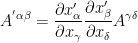
 and
and  (since they occur twice in the term on right). We can illustrate this for 3 dimensional space, i.e.
  but summation performed only on
  and
and  then we have:

 on a plane surface with variable density.
 the density at A, then
  and
and  represent, respectively the partial variation of
  ,
,  in terms of
  will affect “both”
 . We can rewrite this system in condensed form as:
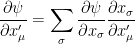
 by
by  and
and  by
by  (to make it similar to notation introduced in case of stress tensor)
 are components of a vector in certain coordinate system. Any set of quantities which transforms according to this equation is defined to be a
 be a vector having two components
  and
and  in a plane and
  be another such vector. If we define
  and
and  (this allows 4 components, namely
  ) with
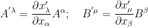
 , then on their addition and multiplication (called
 be a vector having two components
  and
and  in a plane and
  be another such vector. If we define
  and
and  (this allows 4 components, namely
  ) with


 . This is neither a contravarient nor a covariant tensor, hence is rather called a
  indices/superscripts of contravariance and
  indices/subscripts of covariance, such that
  ) and n (having
  indices/superscripts of contravariance and
  indices/subscripts of covariance, such that
  ) respectively, are multiplied together, the result is a
  indices/superscripts of contravariance and
  indices/subscripts of covariance, such that
  ) .
) .
 represents a set of 27 (=3^3) equations with each equation having 27 terms on the right. And the transformation law for tensor
  represents a set of 9 (=3^2) equations with each equation having 9 terms on the right. Therefore, the transformation law of their
  represents a set of 243 (=3^5) equations with each equation having 243 terms on the right.
You must be logged in to post a comment.