Probability Musing

Please let me know if you know the solution to the following problem:

What is the probability of me waking up at 10am?

What additional information should be supplied so as to determine the probability? What do you exactly mean by the probability of this event? Which kind of conditional probability will make sense?

Consider the following comment by Timothy Gowers regarding the model for calculating the probability of an event involving a pair of dice:

Rolling a pair of dice (pp. 6), Mathematics: A very short introduction © Timothy Gowers, 2002 [Source]

I find probability very confusing, for example, this old post.

Childhood Maths – II

I found two documents that I was very proud of as a child. Both were the result of trying to understand the kind of things Ramanujan did in free time, a result of the little AMTI books I read as a child. I will share the second document in this post and the other one was in the previous post.

Following document was created in MS Word on my old Windows XP desktop. The calculations were done using some Microsoft advanced calculator:

I was not happy with the result though since the pattern didn’t continue which was supposed to continue according to Ramanujan.

Childhood Maths – I

I found two documents that I was very proud of as a child. Both were the result of trying to understand the kind of things Ramanujan did in free time, a result of the little AMTI books I read as a child. I will share one document in this post and another one in the next since both are not related to each other in substance.

Following is a calculation table generated using some spreadsheet software:

As you can see, it was motivated by the famous Taxicab number story.

Understanding Geometry – 4

Aleksej Ivanovič Markuševič’s book, “Remarkable Curves” discusses the properties of ellipses, parabolas, hyperbolas, lemniscates, cycloids, brachistochrone, spirals and catenaries.  Among these “lemniscates” are the ones that I encountered only once before starting undergraduate education (all other curves appeared frequently in physics textbooks) and that too just to calculate the area enclosed by this curve. So I will discuss the properties of lemniscates in this post.

Let’s begin with the well-known curve, ellipse. An ellipse is the locus of points whose sum of distances from two fixed points (called foci) is constant. My favourite fact about ellipses is that we can’t find a general formula for the perimeter of an ellipse, and this little fact leads to the magical world of elliptic integrals. This, in turn, leads to the mysterious elliptic functions, which were discovered as inverse functions of elliptic integrals. Further, these functions are needed in the parameterization of certain curves, now called elliptic curves. For more details about this story, read the paper by Adrian Rice and Ezra Brown, “Why Ellipses are not Elliptic curves“.

Lemniscate is defined as the locus of points whose product of distances from two fixed points and (called foci) is constant. Lemniscate means, “with hanging ribbons” in Latin.  If the length of the segment is then for the midpoint of this line segment will lie on the curve if the product constant is . In this case we get a figure-eight lying on its side.

Lemniscate of Bernoulli; By Kmhkmh (Own work) [CC BY 4.0], via Wikimedia Commons

The attempt to calculate the perimeter of the above curve leads to elliptic integral, hence can’t derive a general formula for its perimeter. Just like an ellipse!

If we equate the value of the constant product not to but to another value, the lemniscate will change its shape. When the constant is less than , the lemniscate consists of two ovals, one of which contains inside it the point , and the other the point .

Cassini oval (x^2+y^2)^2−2c^2(x^2−y^2)=a^4−c^4; Source: https://www.encyclopediaofmath.org/legacyimages/common_img/c020700b.gif

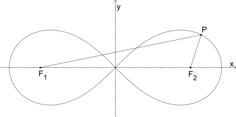
When the product constant is greater than but less than , the lemniscate has the form of a biscuit. If the constant is close to , the “waist” of the biscuit is very narrow and the shape of the curve is very close to the figure-eight shape.

Cassini oval (x^2+y^2)^2−2c^2(x^2−y^2)=a^4−c^4; Source: https://www.encyclopediaofmath.org/legacyimages/common_img/c020700b.gif

If the constant differs little from , the waist is hardly noticeable, and if the constant is equal or greater than the waist disappears completely, and the lemniscate takes the form of an oval.

Cassini oval (x^2+y^2)^2−2c^2(x^2−y^2)=a^4−c^4; Source: https://www.encyclopediaofmath.org/legacyimages/common_img/c020700a.gif

We can further generalize this whole argument to get lemniscate with an arbitrary number of foci, called polynomial lemniscate.

Polynomials and Commutativity

In high school, I came to know about the statement of the fundamental theorem of algebra:

Every polynomial of degree with integer coefficients have exactly complex roots (with appropriate multiplicity).

In high school, a polynomial = a polynomial in one variable. Then last year I learned 3 different proofs of the following statement of the fundamental theorem of algebra [involving, topology, complex analysis and Galois theory]:

Every non-zero, single-variable, degree polynomial with complex coefficients has, counted with multiplicity, exactly complex roots.

A more general statement about the number of roots of a polynomial in one variable is the Factor Theorem:

Let be a commutative ring with identity and let be a polynomial with coefficients in . The element is a root of if and only if divides .

A corollary of above theorem is that:

A polynomial of degree over a field has at most roots in .

(In case you know undergraduate level algebra, recall that is a Principal Ideal Domain if and only if is a field.)

The key fact that many times go unnoticed regarding the number of roots of a given polynomial (in one variable) is that the coefficients/solutions belong to a commutative ring (and is a field hence a commutative ring). The key step in the proof of all above theorems is the fact that the division algorithm holds only in some special commutative rings (like fields). I would like to illustrate my point with the following fact:

The equation has only 2 complex roots, namely and . But if we want solutions over 2×2 matrices (non-commutative set) then we have at least  3 solutions (consider 1 as 2×2 identity matrix and 0 as the 2×2 zero matrix.)

if we allow complex entries. This phenominona can also be illusttrated using a non-commutative number system, like quaternions. For more details refer to this Math.SE discussion.

Four Examples

Following are the four examples of sequences (along with their properties) which can be helpful to gain a better understanding of theorems about sequences (real analysis):

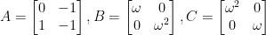
• : unbounded, strictly increasing, diverging
• : bounded, strictly decreasing, converging
• : bounded, strictly increasing, converging
• : bounded, not converging (oscillating)

I was really amazed to found that is a strictly increasing sequence, and in general, the function defined for all positive real numbers is an increasing function bounded by 1:

 

The graph of x/(1+x) for x>0, plotted using SageMath 7.5.1

 

Also, just a passing remark, since for all , and as seen in prime number theorem we get an unbounded increasing function for

The plot of x/log(x) for x>2. The dashed line is y=x for the comparison of growth rate. Plotted using SageMath 7.5.1

 

Prime Polynomial Theorem

I just wanted to point towards a nice theorem, analogous to the Prime Number Theorem, which is not talked about much:

# irreducible monic polynomials with coefficients in and of degree , for a prime power .

The proof of this theorem follows from Gauss’ formula:

# monic irreducible polynomialswith coefficients in and of degree = , by taking .

 

For details, see first section of this: http://alpha.math.uga.edu/~pollack/thesis/thesis-final.pdf

Recursion and Periodicity

One of the simplest recursive formula that I can think of is the one which generates the Fibonacci sequence, with . So, I will illustrate a following general concept about recursions using Fibonacci sequence.

A sequence generated by a recursive formula is periodic modulo k, for any positive integer k greater than 1.

I find this fact very interesting because it means that a sequence which is strictly increasing when made bounded using the modulo operation (since it will allow only limited numbers as the output of recursion relation), will lead to a periodic cycle.

Following are the first 25 terms of the Fibonacci sequence:

1, 1, 2, 3, 5, 8, 13, 21, 34, 55, 89, 144, 233, 377, 610, 987, 1597, 2584, 4181, 6765, 10946, 17711, 28657, 46368, 75025.

And here are few examples modulo k, for k=2,3,4,5,6,7,8

As you can see, the sequence repeats as soon as 1,0 appears. And from here actually one can see why there should be a periodicity.

For the sequence to repeat, what we need is a repetition of two consecutive values (i.e. the number of terms involved in the recursive formula) in the sequence of successive pairs. And for mod k, the choices are limited, namely k^2.  Now, all we have to ensure is that “1,0” should repeat. But since consecutive pairs can’ repeat (as per recursive formula) the repetition of “1,0” must occur within the first k^2.

For rigorous proofs and its relation to number theory, see: http://math.stanford.edu/~brianrl/notes/fibonacci.pdf

Repelling Numbers

An important fact in the theory of prime numbers is the Deuring-Heilbronn phenomenon, which roughly says that:

The zeros of L-functions repel each other.

Interestingly, Andrew Granville in his article for The Princeton Companion to Mathematics remarks that:

This phenomenon is akin to the fact that different algebraic numbers repel one another, part of the basis of the subject of Diophantine approximation.

I am amazed by this repelling relation between two different aspects of arithmetic (a.k.a. number theory). Since I have already discussed the post Colourful Complex Functions, wanted to share this picture of the algebraic numbers in the complex plane, made by David Moore based on earlier work by Stephen J. Brooks:

Source: http://blogs.ams.org/visualinsight/2013/09/01/algebraic-numbers/

 

In this picture, the colour of a point indicates the degree of the polynomial of which it’s a root, where red represents the roots of linear polynomials, i.e. rational numbers,  green represents the roots of quadratic polynomials, blue represents the roots of cubic polynomials, yellow represents the roots of quartic polynomials, and so on.  Also, the size of a point decreases exponentially with the complexity of the simplest polynomial with integer coefficient of which it’s a root, where the complexity is the sum of the absolute values of the coefficients of that polynomial.

Moreover,  John Baez comments in his blog post that:

There are many patterns in this picture that call for an explanation! For example, look near the point . Can you describe some of these patterns, formulate some conjectures about them, and prove some theorems? Maybe you can dream up a stronger version of Roth’s theorem, which says roughly that algebraic numbers tend to ‘repel’ rational numbers of low complexity.

To read more about complex plane plots of families of polynomials, see this write-up by John Baez. I will end this post with the following GIF from Reddit (click on it for details):

So I heard you guys like rotating roots of polynomials in the complex plane…
byu/turnipheadscarecrow inmath

Prime Consequences

Most of us are aware of the following consequence of Fundamental Theorem of Arithmetic:

There are infinitely many prime numbers.

The classic proof by Euclid is easy to follow. But I wanted to share the following two analytic equivalents (infinite series and infinite products) of the above purely arithmetical statement:

•   diverges.

For proof, refer to this discussion: https://math.stackexchange.com/q/361308/214604

• , where is any complex number with .

The outline of proof,   when is a real number, has been discussed here: http://mathworld.wolfram.com/EulerProduct.html