Monthly Archives: April 2017

Understanding Geometry – 2

Standard

If you want to brush up your high school geometry knowledge, then KhanAcademy is a good place to start. For example, I learned a new proof of Pythagoras Theorem (there are 4 different proofs on KhanAcademy) which uses scissors-congruence:

In this post, I will share with you few theorems from L. I. Golovina and I. M. Yaglom’s “Induction in Geometry ”  which I learned while trying to prove Midpoint-Polygon Conjecture.

Theorem 1: The sum of interior angles of an n-gon is 2\pi (n-2).

Theorem 2: The number of ways in which a convex n-gon can be divided into triangles by non-intersecting diagonals is given by
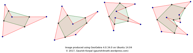
\displaystyle{\frac{2(2n-5)!}{(n-1)!(n-3)!}}

Theorem 3: Given a \triangle ABC, with n-1 straight lines CM_1, CM_2, \ldots CM_{n-1} drawn through its vertex C, cutting the triangle into n smaller triangles \triangle ACM_1, \triangle M_1CM_2, \ldots, \triangle M_{n-1}CB. Denote by r_1, r_2, \ldots r_n and \rho_1, \rho_2, \ldots, \rho_n respectively the radii of the inscribed and circumscribed circles of these triangles (all the circumscribed circles are inscribed within the angle C of the triangle) and let r and \rho be the radii of the inscribed and circumscribed circles (respectively) of the \triangle ABC itself. Then

\displaystyle{\frac{r_1}{\rho_1} \cdot\frac{r_2}{\rho_2} \cdots\frac{r_n}{\rho_n} =\frac{r}{\rho} }

Theorem 4: Any convex n-gon which is not a parallelogram can be enclosed by a triangle whose sides lie along three sides of the given n-gon.

Theorem 5 (Levi’s Theorem): Any convex polygon which is not a parallelogram can be covered with three homothetic polygons smaller than the given one.

The above theorem gives a good idea of what “combinatorial geometry” is all about. In this subject, the method of mathematical induction is widely used for proving various theorems. Combinatorial geometry deals with problems, connected with finite configurations of points or figures. In these problems, values are estimated connected with configurations of figures (or points) which are optimal in some sense.

Theorem 6 (Newton’s Theorem): The midpoints of the diagonals of a quadrilateral circumscribed about a circle lie on one straight line passing through the centre of the circle.

Theorem 7 (Simson’s Theorem): Given a \triangle ABC inscribed in the circle S with an arbitrary point P on this circle. Then then feet of the perpendiculars dropped from the point P to the sides of the \triangle ABC are collinear.

We can extend the above idea of Simson’s line to any n-gon inscribed in a circle.

Theorem 8: A 3-dimensional space is divided into \frac{(n+1)(n^2-n+6)}{6} parts by n planes, each three of which intersect and no four of which have a common point.

Theorem 9: Given n spheres in 3-dimesnional space, each four of which intersect. Then all these spheres intersect, i. e. there exists a point belonging to all the spheres.

Theorem 10 (Young’s Theorem): Given n points in the plane such that each pair of them are at a distance of at most 1 from each other. Then all these points can be enclosed in a circle of radius 1/\sqrt{3}.

I won’t be discussing their proofs since the booklet containing the proofs and the detailed discussion is freely available at Mir Books.

Also, I would like to make a passing remark about the existence of a different kind of geometry system, called “finite geometry“. A finite geometry is any geometric system that has only a finite number of points. The familiar Euclidean geometry is not finite because a Euclidean line contains infinitely many points. A geometry based on the graphics displayed on a computer screen, where the pixels are considered to be the points, would be a finite geometry. While there are many systems that could be called finite geometries, attention is mostly paid to the finite projective and affine spaces because of their regularity and simplicity. You can learn more about it here: http://www.ams.org/samplings/feature-column/fcarc-finitegeometries

Huntington’s Red-Blue Set

Standard

While reading Lillian Lieber’s book on infinity, I came across an astonishing example of infinite set (on pp. 207). Let’s call the property of existence of a rational number between given two rational number to be “beauty” (a random word introduced by me to make arguments clearer).

The set of rational numbers between 0 and 1 are arranged in ascending order of magnitude, and all of them are coloured blue. This is clearly a beautiful set. Then another another set of rational numbers between 0 and 1 is taken and arrange in ascending order of magnitude, but all of them are coloured red. This is also a beautiful set. Now, put these two sets together in such a way that each blue number is immediately followed by the corresponding red number. For example, 1/2 is immediately followed by 1/2 etc.  It appears that if we interlace two beautiful sets, the resulting set should be even more beautiful. But since each blue number has an immediate successor, namely the corresponding red number, so that between these two we can’t find even a single other rational number, red or blue, the resulting set is NOT beautiful.

The set created above is called Huntington’s Red-Blue set. It is an ingenious invention, where two beautiful sets combined together lead to loss of beauty. For more details, read the original paper:

Huntington, Edward V. “The Continuum as A Type of Order: An Exposition of the Modern Theory.” Annals of Mathematics, Second Series, 7, no. 1 (1905): 15-43. doi:10.2307/1967192.

Understanding Geometry – 1

Standard

When we think about mathematics, what comes to our mind are the numbers and figures. The  study of numbers is called arithmetic and the study of figures is called geometry (in very crude sense!). In our high school (including olympiad level) and college curriculum we cover various aspects of arithmetic. I am very much satisfied with that treatment, and this is the primary reason for my research interests in arithmetic (a.k.a. number theory).

But, I was always unsatisfied with the treatment given to geometry in our high school curriculum. We were taught some plane Euclidean geometry (with the mention of the existence of non-euclidean geometries), ruler and compass constructions, plane trigonometry (luckily, law of cosines was taught), surface area & volume of 3D objects, 2D coordinate geometry, conic sections and 3D coordinate geometry.  In the name of Euclidean geometry some simple theorems for triangles, quadrilaterals and circles are discussed, like triangle congruence criterias, triangle similarity criterias, Pythagoras theorem, Mid-Point Theorem, Basic Proportionality Theorem, Thales’ Theorem, Ptolemy’s theorem, Brahmagupta theorem etc. are discussed. Ruler-compass constructions are taught as “practical geometry”. Students are asked to cram the formulas of area (including Brahmagupta’s formula and Heron’s formula) and volume without giving any logic (though in earlier curriculum teacher used to give the reasoning). Once coordinate geometry is introduced, students are asked to forget the idea of Euclidean geometry or visualizing 3D space. And to emphasize this, conic sections are introduced only as equations of curves in two dimensional euclidean plane.

The interesting theorems from Euclidean geometry like Ceva’s theorem,  Stewart’s Theorem,  Butterfly theorem, Morley’s theorem (I discussed this last year with high school students), Menelaus’ theorem, Pappus’s theorem,  etc. are never discussed in classroom (I came to know about them while preparing for olympiads). Ruler-compass constructions are taught without mentioning the three fundamental impossibilities of angle trisection, squaring a circle and doubling a cube. The conic sections are taught without discussing the classical treatment of the subject by Apollonius.

In the classic “Geometry and Imagination“, the first chapter on conic sections is followed by discussion of crystallographic groups (Character tables for point groups),  projective geometry (recently I discussed an exciting theorem related to this) and differential geometry (currently I am doing an introductory course on it). So over the next few months I will be posting mostly about geometry (I don’t know how many posts in total…), in an attempt to fill the gap between high-school geometry and college geometry.

I agree with the belief that algebraic and analytic methods make the handling of geometry problems much easier, but in my opinion these methods suppress the visualization of geometric objects. I will end this introductory post with a way to classify geometry by counting the number of ideal points in projective plane:

  • Hyperbolic Geometry (a.k.a. Lobachevsky-Bolyai-Gauss type non-euclidean geometry) which has two ideal points [angle-sum of a triangle is less than 180°].
  • Elliptic Geometry (a.k.a. Riemann type non-euclidean geometry) which has no ideal points. [angle-sum of a triangle is more than 180°]
  • Parabolic Geometry (a.k.a. euclidean geometry)  which has one ideal point. [angle-sum of a triangle is 180°]

Midpoint Polygon Conjecture is false

Standard

Contrary to my expectations, my previous post turned out to be like  Popular-­Lonely primes and Decimal Problem, i.e. I discovered nothing new.

My conjecture is false. Following counterexample is given on pp. 234 of this paper:

poly-counter

Counterexample of the conjecture, taken from: Berlekamp, E. R., E. N. Gilbert, and F. W. Sinden. “A Polygon Problem.” The American Mathematical Monthly 72, no. 3 (1965): 233-41. doi:10.2307/2313689.

As pointed out by uncombed_coconut, the correct theorem is:

Theorem (Berlekamp-Gilbert-Sinden, 1965). For almost all simple polygons there exist a smallest natural number k such that after k iterations of midpoint polygon procedure, we obtain a convex polygon.

The proof of this theorem is very interesting. Till now I thought that proving euclidean geometry theorems using complex numbers was an overkill. But using an N-tuple of complex numbers to represent the vertices of a closed polygon (in given order),  \mathbf{z} = (z_1,\ldots , z_N),  we can restate the problem in terms of eigenvectors (referred to as eigenpolygons) and eigenvalues.  Following are the crucial facts used is the proof:

  • An arbitrary N-gon (need not be simple) can be written as a sum of regular N-gons i.e. the eigenvalues are distinct.
  • The coefficient of k^{th} eigenvector (when N-gon is written as linear combination of eigenpolygons) is the centroid of the polygon obtained by “winding” \mathbf{z} k times.
  • All vertices of the midpoint polygons (obtained by repeating the midpoint polygon procedure infinitely many times) converge to the centroid.
  • The sum of two convex components of \mathbf{z} is a polygon. This polygon is the affine image of a regular convex N-gon whose all vertices lie on an ellipse. (as pointed out by Nikhil)
  • A necessary and sufficient condition for \mathbf{z} to have a convex midpoint polygon (after some finite iterations of the midpoint polygon procedure) is that the ellipse circumscribing the sum of two convex components of \mathbf{z} is nondegenerate. (The degenerate form of an ellipse is a point. )

For a nice outline of the proof, please refer to the comment by uncombed_coconut on previous post.

Since I didn’t know that this is a well studied problem (and that too by a well known mathematician!) I was trying to prove it on my own. Though I didn’t make much progress, but I discovered some interesting theorems which I will share in my future posts.

Midpoint Polygon Conjecture

Standard

This is going to be yet another ambitious post like New Diagonal Contribution Theorem, and Cross Diagonal Cover Problem.

Let’s begin with following definitions from Wikipedia:

A convex polygon is a simple polygon (not self-intersecting) in which no line segment between two points on the boundary ever goes outside the polygon.

A concave polygon is a simple polygon (not self-intersecting) which has at least one reflex interior angle – that is, an angle with a measure that is between 180 degrees and 360 degrees exclusive.

We know that 3 sided polygons (a.k.a triangles) are always convex.  So, they are not very interesting. Let’s define the following procedure:

Midpoint Polygon Procedure: Given a n-sided simple polygon, join the consecutive midpoints of the sides to generate another n-sided simple polygon.

Here are few examples:

concave-convex

Red polygon is the original polygon, green polygon is the one generated by joining midpoints.

We observe that if the original polygon was a concave polygon then the polygon generated by joining midpoints need not be a convex polygon. So, let’s try to observe what happens when we apply the midpoint polygon procedure iteratively on the 4th case above (i.e. when we didn’t get a convex polygon):

big-gon

In fourth iteration of the described procedure, we get the convex polygon.

Based on this observation, I want to make following conjecture:

Midpoint Polygon Conjecture: For every simple polygon there exists a smallest natural number k such that after k iterations of midpoint polygon procedure, we obtain a convex polygon.

If the given polygon is convex, then there is nothing to prove since k=1, but I have no idea about how to prove it for concave polygons. I tried to Google for the answer, but couldn’t find anything similar. So, if you know the proof or counterexample of this conjecture, please let me know.